One Dimensional Non-Continuous Motion
In continuous motion, we used a single mathematical function each to describe the position, velocity, or acceleration over time. If we cannot describe the motion with a single mathematical function over the entire time period, that motion is considered non-continuous motion. In cases such as this we will use different equations for different sections of the overall time period.
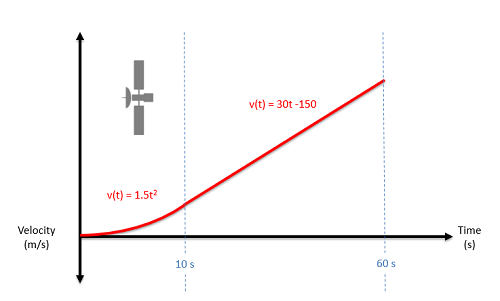
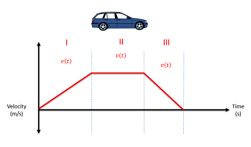
For an example of non-continuous motion, imagine a car that accelerates for a few seconds, then holds a steady speed for a few seconds, then puts on the brakes and comes to a stop over the final few seconds. There is no one mathematical function we can use to describe the motion for the full time period, but if we break the motion into three pieces, then we can come up with an equation for each section of the motion.
Analyzing the first time period will be exactly the same as analyzing a continuous function. We will initially need to identify the mathematical function to describe position, or velocity, or acceleration for that first time period. Next we take derivatives to move from position to velocity to acceleration or take integrals to move from acceleration to velocity to position. Whenever we take an integral, we need to remember to include the constant of integration which will represent the initial velocity or the initial position (in the velocity and position equations respectively).
For the second, third (and all following) sections, we will do much the same process. We will start by identifying an equation for the position, or velocity, or acceleration for that time period. From there we again take derivatives or integrals as appropriate, but now the constants of integration will be a little more complicated. Those constants still represent initial velocities and and positions in a sense, but they will be the velocity and position when t=0, not the velocity and position at the start of that section.
To find the constants of integration, we are instead going to have to use the transition point, which is the point in time where we are moving from one set of equations to the next. Even though the equations are changing, we cannot have an instantaneous jump in either the position or velocity. An instantaneous jump in either position or velocity would require infinite acceleration, which is physically impossible.
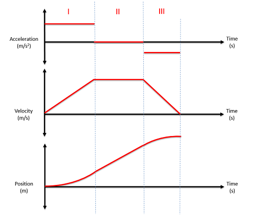
To find the velocity equations for the second time frame (or third or fourth etc.), we start by integrating the acceleration equation for that same time period. This will lead to an equation with an unknown constant of integration. To solve for that constant we look back to the velocity equation for the previous time frame and solve for the velocity at the very end of this prior time period. Since it can't jump instantaneously, this is also the velocity at the start of the current time period. Using this velocity, along with the time t at the transition point, we can solve for the last unknown in the current velocity equation (the constant of integration).
To find the position equation for the second time frame (or third or fourth etc.), we start by integrating the velocity equation for the same time period (you will need to solve for the unknowns in the velocity equation first, as discussed above). After integration, we should have one new constant of integration in the position equation. Just as we did with the velocity equations, we will use the position equation from the prior time frame to solve for the position at the transition point, then use that value along with the known time t to solve for the unknown constant in the current position equation.