Dependent Motion in Particles
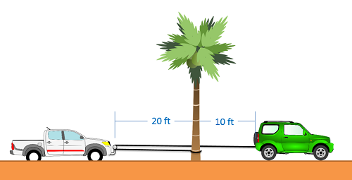
Dependent motion analysis is used when two or more particles have motions that are in some way connected to one another. The way in which the motion of these particles is connected is known as the constraint. A simple example of a constrained system is shown in the image below. Imagine a pickup truck gets stuck in the sand, and a friend uses a rope to help pull them out. This friend ties one end of the rope to the rear bumper of her car, loops the rope around a bar on the front of the pickup truck, then ties the other end to a stationary tree. In this case the two vehicles will not have the same velocity or acceleration, but their motions are related because they are tied together by the rope. In this case, the rope is acting as the constraint, allowing us to know the velocity or acceleration of one vehicle based on the velocity or acceleration of the other vehicle.
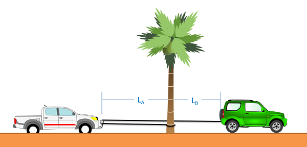
The first thing we will need to do when analyzing these systems is to come up with what is known as the constraint equation. A constraint equation will be some geometric relationship that will remain true over the course of the motion. In the above example, imagine the rope is 50 ft long. Using the tree as a stationary point, we can also say that the length of the rope is the distance from the green car to the tree, plus two times the distance from the pickup truck to the tree (since it must go out to the pickup truck and then back). If we put this into an equation (the constraint equation) we would have the following.
| Constraint Equation: Positions | \[L= 50 ft = 2 L_{A}+L_{B}\] |
|---|
Once we have a constraint equation that works for positions, we can take the derivative of this equation to find another constraint equation that relates velocities. In this case, the length of the rope is constant, and therefore the derivative of the length will be zero. If we take the derivative of the constraint equation again, we wind up with a third constraint equation that relates accelerations.
| Constraint Equation: Velocities | \[\dot{L}=0=2 \dot{L}_{A}+\dot{L}_{B}\] |
|---|---|
| Constraint Equation: Accelerations | \[\ddot{L}=0=2 \ddot{L}_{A}+\ddot{L}_{B}\] |
In these equations, it is important to remember that the values represent the changes in length, rather than direct measures of velocities. Though both vehicles would have positive velocities in the example above (velocities to the right), one L dot value will be positive and one will be negative. This is because the truck is getting closer to the tree while the green car is getting further away. A similar situation will occur for the accelerations, where both vehicles would have positive accelerations even if the L double dot values are a mix of positive and negative values.