Viscous Damped Free Vibrations
Viscous damping is damping that is proportional to the velocity of the system. That is, the faster the mass is moving, the more damping force is resisting that motion. Fluids like air or water generate viscous drag forces.
We will only consider linear viscous dampers, that is where the damping force is linearly proportional to velocity. The equation for the force or moment produced by the damper, in either x or θ, is:
| \[ \vec{F{_c}} =c \vec{\dot{x}} \] |
| \[\vec{M{_c}} =c \vec{\dot{\theta}} \] |
Where c is the damping constant, which is a physical property of the damper (based on type of fluid, size of piston, etc.). Note that the units of c change depending on whether it is damps linear (N-s/m) or rotational motion (N-m s/rad).
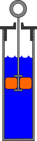
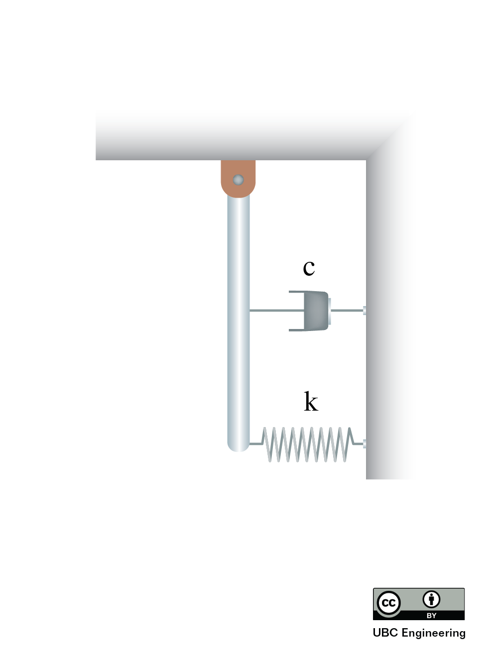
When the system is at rest in the equilibrium position, the damper produced no force on the system (no velocity), while the spring can produce force on the system, such as in the hanging mass shown above. Recall that this is the equilibrium position, but the spring is NOT at its unstretched length, as the static mass produces an extention of the spring.
If we perturb the system (applying an initial displacement, or an initial velocity, or both), the system will tend to move back to its equilibrium position. What that movement looks like will depend on the system parameters (m, c, and k).
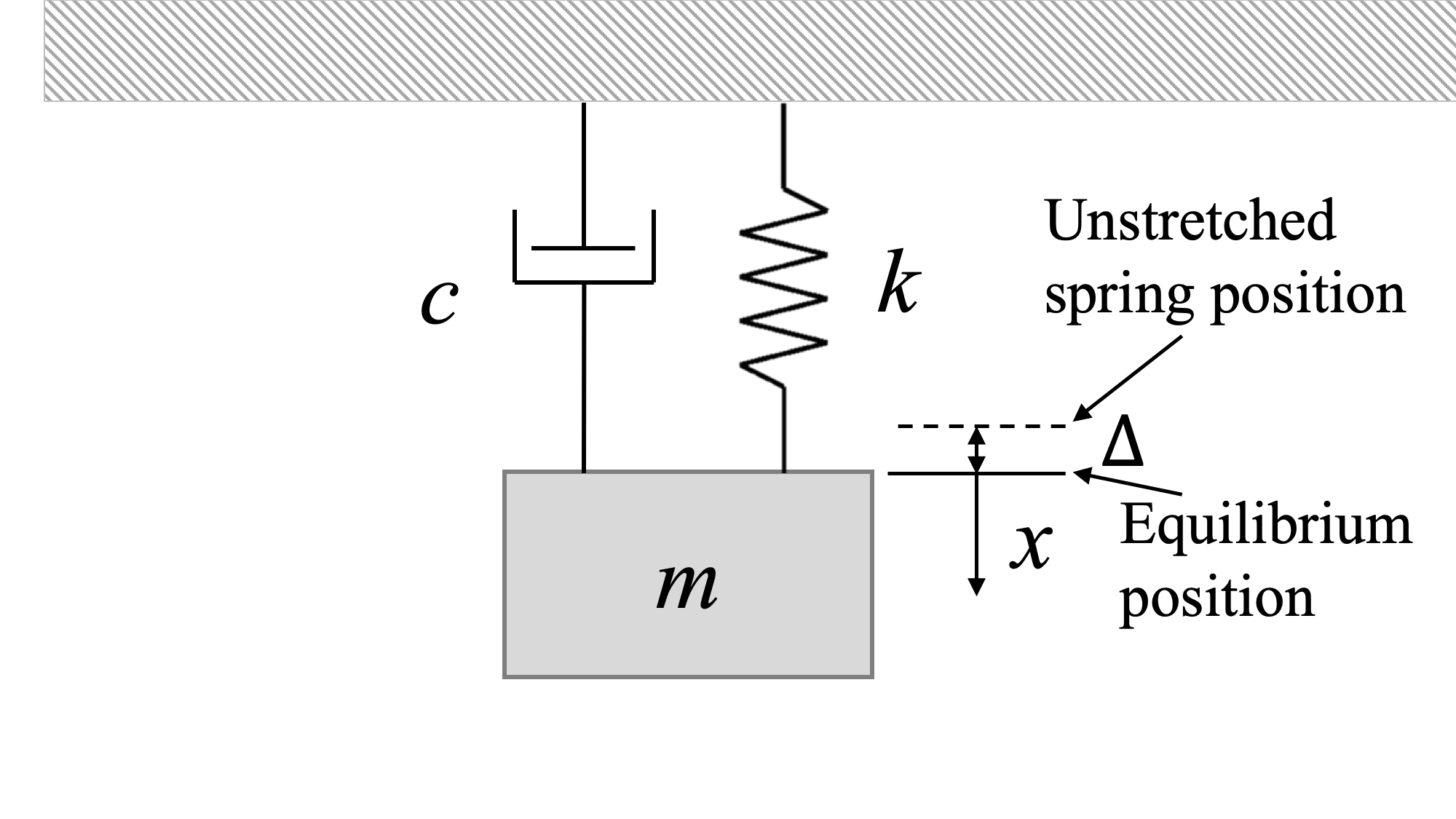
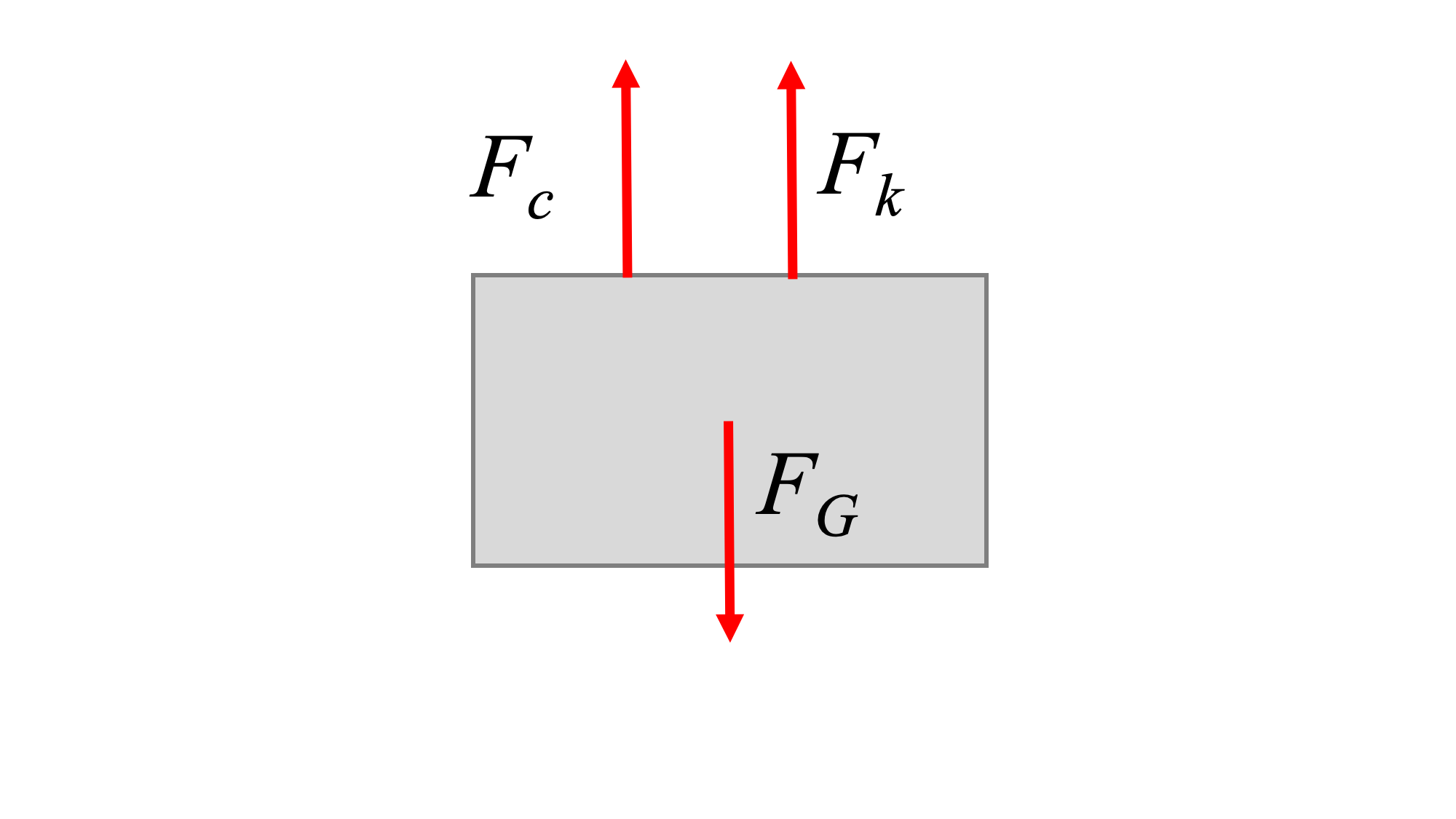
To determine the equation of motion of the system, we draw a free-body diagram of the system with perturbation and apply Newton's second law.
The process for finding the equation of motion of the system is again:
- Sketch the system with a small positive perturbation (x or θ).
- Draw the free-body diagram of the perturbed system. Ensure that the spring force and the damper force have directions opposing the perturbation.
- Find the one equation of motion for the system in the perturbed coordinate using Newton's Second Law. Keep the same positive direction for position, and assign positive acceleration in the same direction.
- Move all terms of the equation to one side, and check that all terms are positive. If all terms are not positive, there is an error in the direction of displacement, acceleration, and/or spring or damper force.
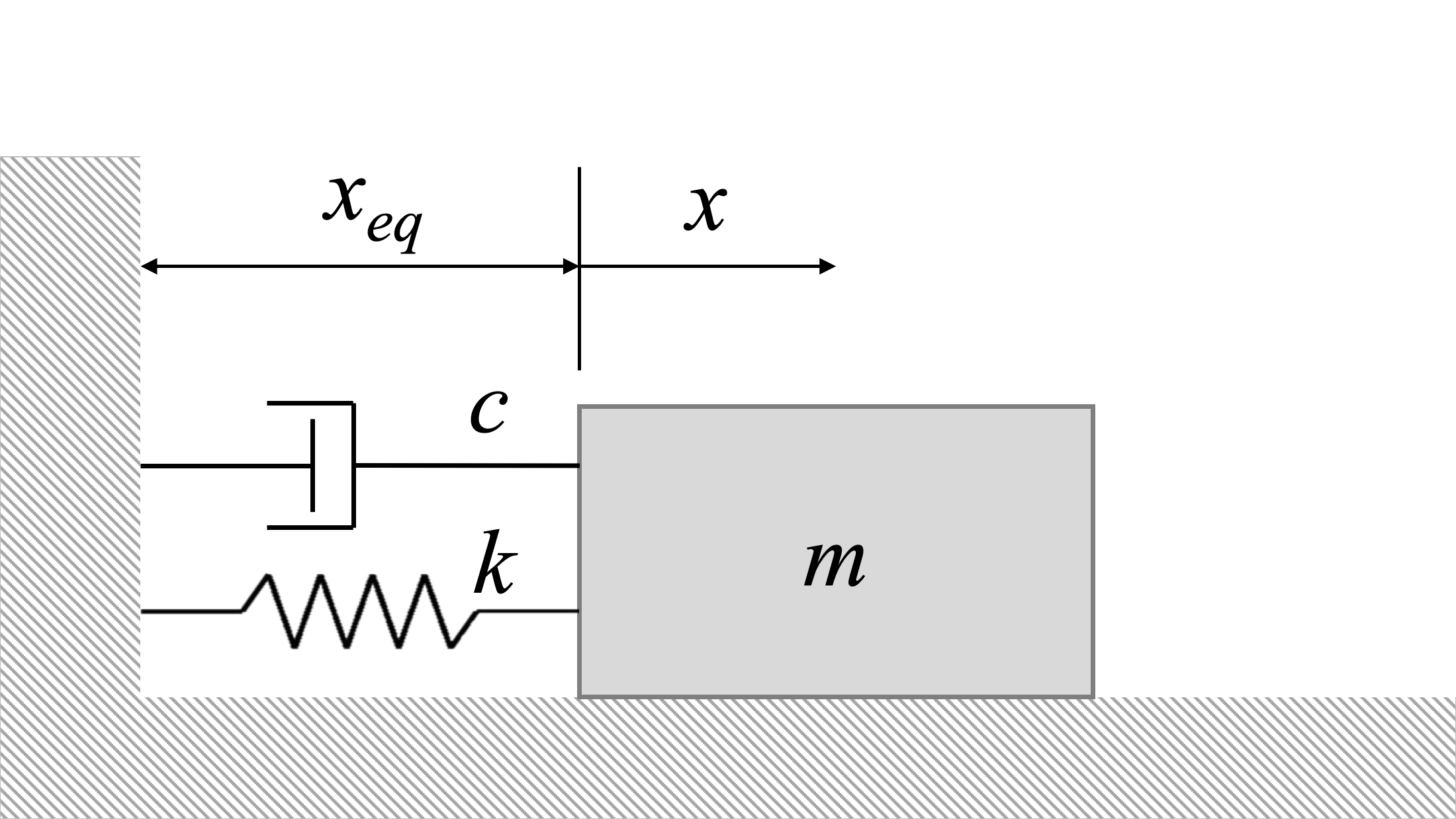
For the example system above, with mass m, spring constant k and damping constant c, we derive the following:
| \[ \sum F_x = m a_x = m {\ddot{x}} \] |
| \[ -F_k - F_c = m {\ddot{x}} \] |
| \[ -k x - c \dot(x) = m {\ddot{x}} \] |
| \[ m {\ddot{x}} + c \dot(x) + k x = 0 \] |
This gives us a differential equation that describes the motion of the system. We can rewrite it in normal form:
| \[ m {\ddot{x}} + c \dot{x} + k {x} = 0 \] |
| \[ \Rightarrow \, {\ddot{x}} + \frac{c}{m} \dot{x} + \frac{k}{m} {x} = 0 \] |
| \[ \Rightarrow \, {\ddot{x}} + 2 \zeta \omega_n \dot{x} + \omega_n^2 {x} = 0 \] |
As before, the term ωn is called the angular natural frequency of the system, and has units of rads/s.
| \[ \omega_n^2 = \frac{k}{m} \] |
| \[ \omega_n = \sqrt{\frac{k}{m}} \] |
ζ (zeta) is called the damping ratio. It is a dimensionless term that indicates the level of damping, and therefore the type of motion of the damped system.
| \[ \zeta = \frac{c}{c_c} \] |
| \[ \zeta = \frac{\text{actual damping}}{\text{critical damping}} \] |
The expression for critical damping comes from the solution of the differential equation. The solution to the system differential equation is of the form:
| \[ x(t) = ae^{rt} \] |
Where a is a constant, and the value(s) of r can be obtained by differentiating this general form of the solution and substituting into the equation of motion.
| \[ m r^2 e^{rt} + c r e^{rt} + k e^{rt} = 0 \] |
| \[ \Rightarrow (m r^2 + c r + k ) e^{rt} = 0 \] |
Because the exponential term is never zero, we can divide both sides by that term and get:
| \[ m r^2 + c r + k = 0 \] |
Using the quadratic formula, we can find the roots of the equation:
| \[ r_{1,2} = (\frac{-c \pm \sqrt{c^2 - 4mk}}{2m}) \] |
Critical damping occurs when the term under the square root sign equals zero:
| \[ c_c^2 = 4 m k \] |
| \[ c_c = 2 \sqrt{m k} = 2m \omega_n \] |
Four Viscous Damping Cases
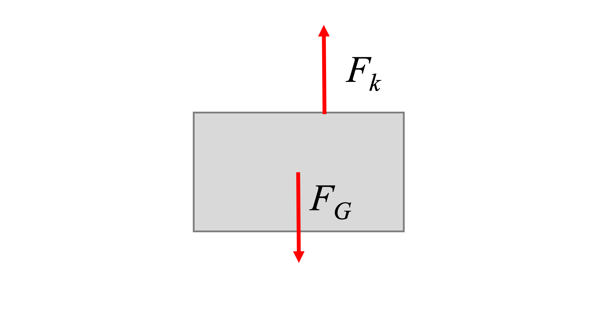
There are four basic cases for the damping ratio. For the solutions that follow in each case, we will assume that the initial perturbaion displacement of the system is x0 and the initial perturbation velocity of the system is v0.
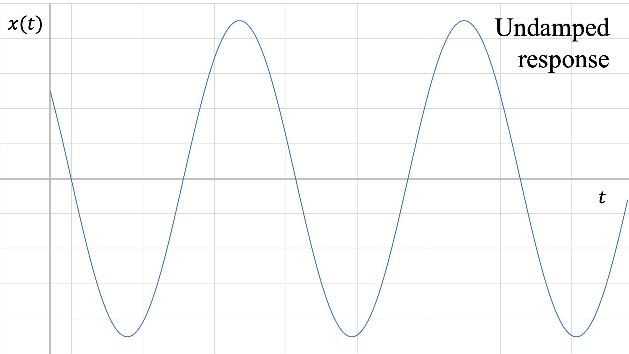
1. ζ = 0: Undamped.
| \[ c =0 \] |
This is the case covered in the previous section. Undamped systems oscillate about the equilibrium position continuously, unless some other force is applied.
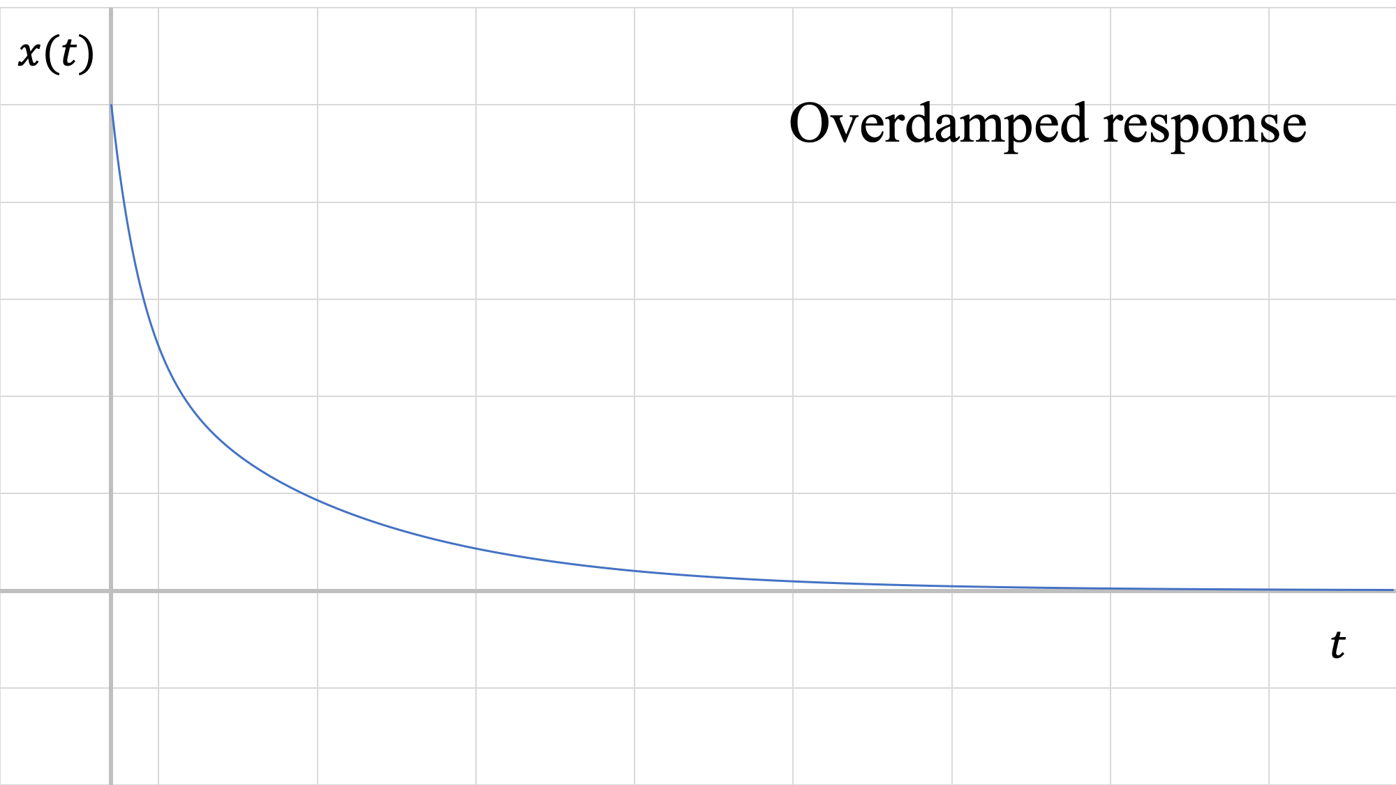
2. ζ > 1: Overdamped.
| \[ c^2 > 4mk \] |
Roots are both real and negative, but not equal to each other. Overdamped systems move slowly toward equilibrium without oscillating.
The solution for an overdamped system is:
| \[ x(t) = a_1 e^{(\frac{-c + \sqrt{c^2 - 4mk}}{2m} ) t} + a_2 e^{(\frac{-c - \sqrt{c^2 - 4mk}}{2m} ) t} \] |
Where:
| \[ a_1 = \frac{-v_0 + r_2 x_0}{r_2 - r_1} \] |
| \[ a_2 = \frac{v_0 + r_1 x_0}{r_2 - r_1} \] |
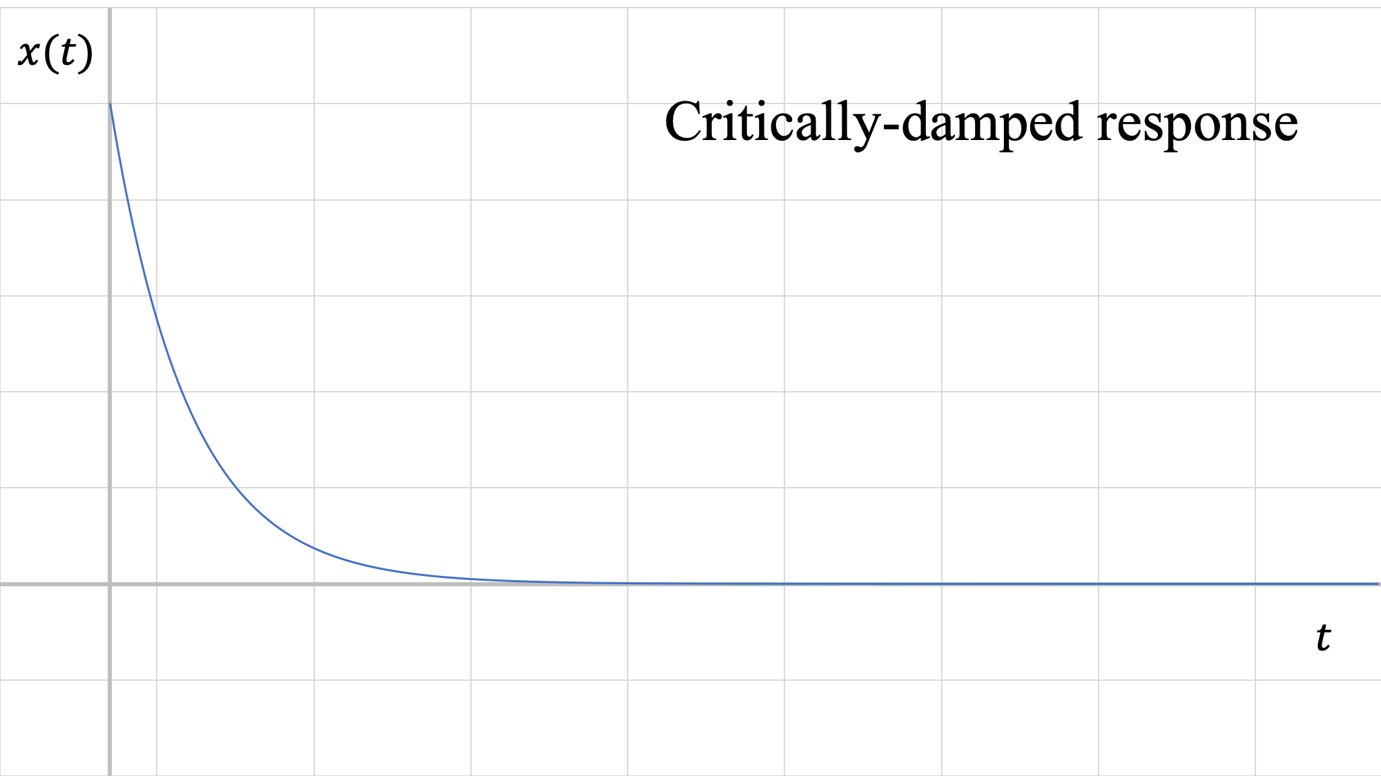
3. ζ = 1: Critically-damped.
| \[ c^2 = 4mk \, (=c_c^2) \] |
Roots are real and both equal to -ωn. Critically-damped systems will allow the fastest return to equilibrium without oscillation.
The solution for a critically-damped system is:
| \[ x(t) = (A + Bt) e^{-\omega_n t} \] |
Where:
| \[ A = x_0\] |
| \[ B = v_0 + x_0 \omega_n\] |
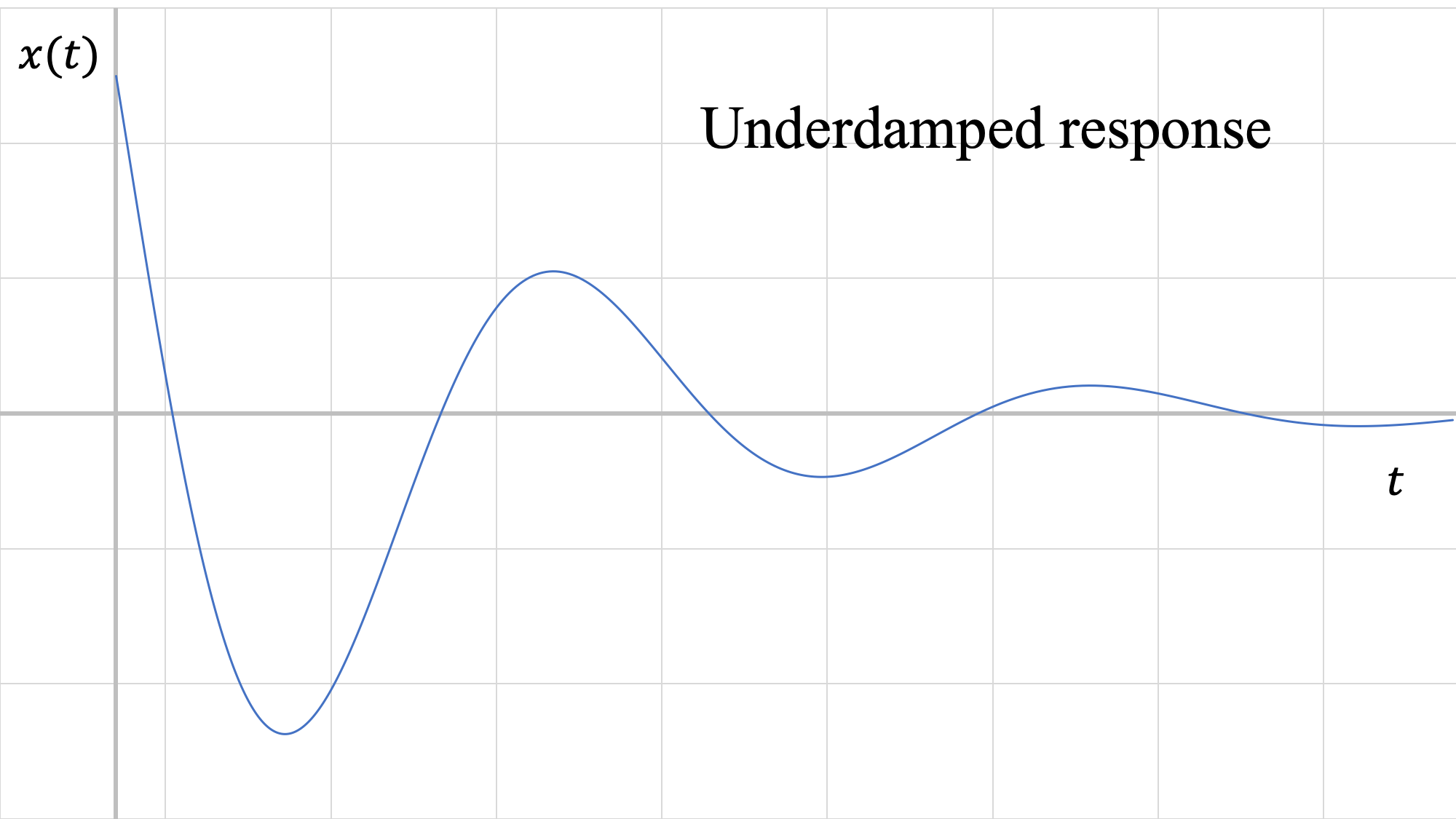
4. ζ < 1: Underdamped.
| \[ c^2 < 4mk \] |
The roots are complex numbers. Underdamped systems do oscillate around the equilibrium point. Unlike undamped systems, the amplitude of the oscillations diminishes until the system eventually stops moving at the equilibrium position.
The solution for an underdamped system is:
| \[ x(t) = \lbrack C_1 \sin (\omega_d t) + C_2 \cos(\omega_d t) \rbrack e^{-\omega_n \zeta t} \] |
Where:
| \[ C_1 = \frac{v_0 + \omega_n \zeta x_0}{\omega_d}\] |
| \[ C_2 = x_0\] |
| \[ \zeta = \frac{c}{2m \omega_n}\] |
This can alternately be expressed as:
| \[ x(t) = A \sin (\omega_d t + \phi) e^{-\omega_n \zeta t}\] |
Where:
| \[ A = \sqrt{\frac{(v_0 + \omega_n \zeta x_0)^2 +(x_0 \omega_d)^2}{\omega_d^2}} \] |
| \[ \phi = \tan^-1 \left( \frac{x_0 \omega_d}{v_0 + \omega_n \zeta x_0}\right)\] |
| \[ \zeta = \frac{c}{2m \omega_n}\] |
ωd is called the damped natural frequency of the system. It is always less than ωn:
| \[ \omega_d = \sqrt{1-\zeta^2} \omega_n \] |
The period of the underdamped response differs from the undamped response as well.
| \[ \text{Undamped: } \tau_n = \frac{2 \pi}{\omega_n} \] |
| \[ \text{Underdamped: } \tau_d = \frac{2 \pi}{\omega_d} \] |
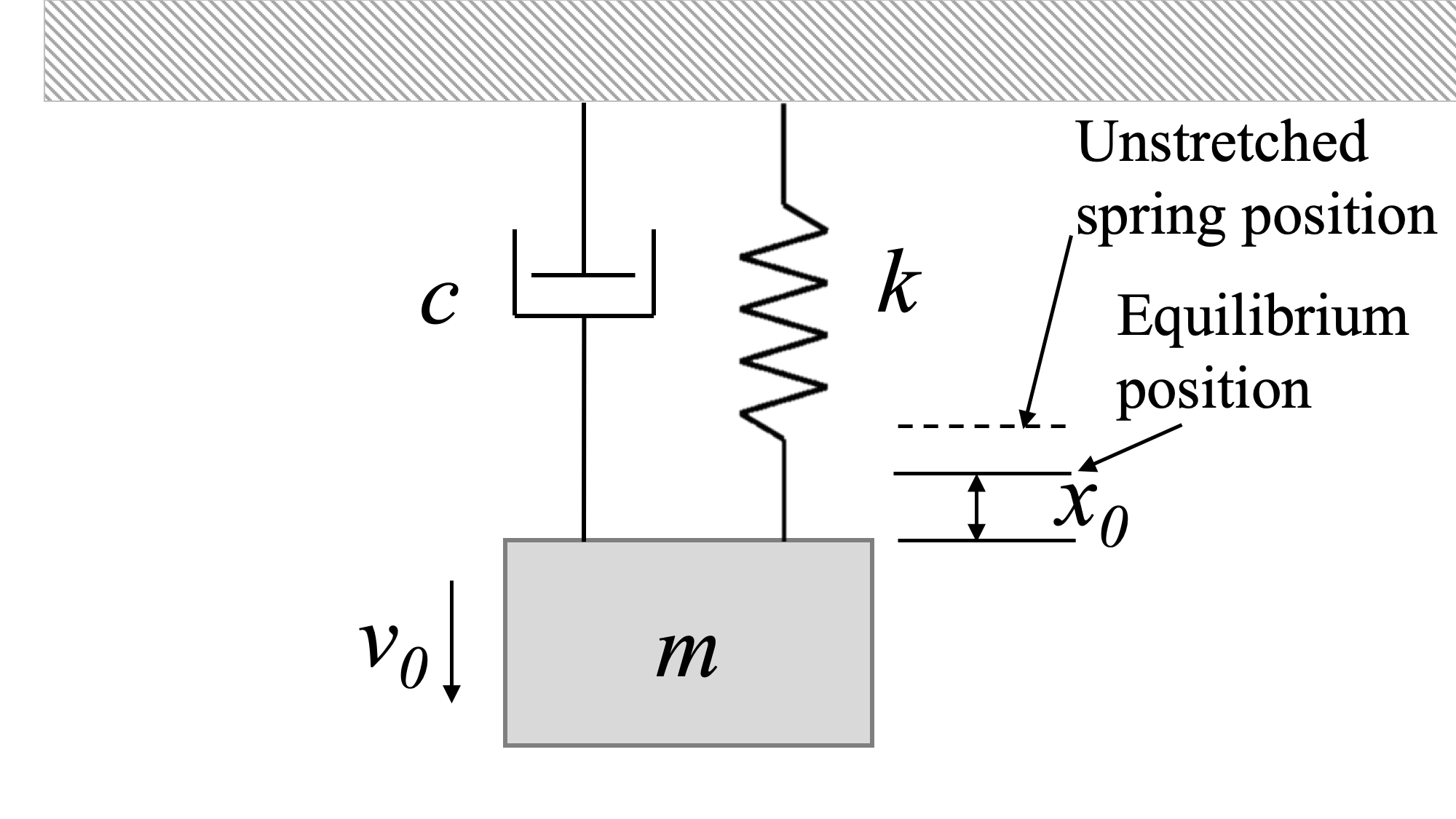
Comparison of Viscous Damping Cases
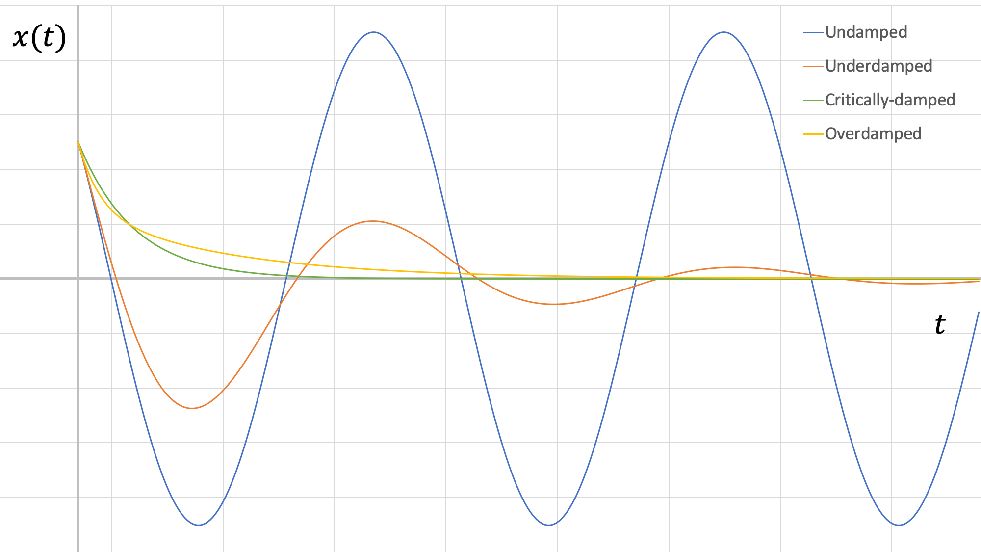
In the figure above, we can see that the critically-damped response results in the system returning to equilibrium the fastest. Also, we can see that the underdamped system amplitude is quite attenuated compared to the undamped case.